Model Analysis Report

Generated: 2026-04-24 21:06:23 Total Models: 9 trained models

Abstract

This report presents a comprehensive analysis of multiple deep learning models developed for extrachromosomal DNA (ecDNA) prediction. The models were trained on a large-scale dataset with severe class imbalance and evaluated using multiple performance metrics including auPRC, AUC, Precision, Recall, and F1-score.

Dataset Description

Sample Distribution

Dataset	Total Samples	Positive Samples	Positive Rate
Training	308	234	75.9740%
Validation	38	29	76.3158%
Test	40	31	77.5000%

Total: 386 samples, 294 positive (76.1658%)

Note: The dataset has a high positive rate (~76%). This is expected as samples were pre-selected based on ecDNA presence for model training.

Model Architecture Comparison

Overview

Model	Architecture	Network Structure	Loss Function	Optimizer
baseline_mlp	BaselineMLP	57→128→64→1	BCEWithLogitsLoss	Adam
deep_residual	DeepResidual	57→128(ResNet)→1	BCEWithLogitsLoss	AdamW
dgit_super	DGITSuper	57→192→Transformer(3 layers)→1	MultiTaskFocalLoss	AdamW
optimized_residual	OptimizedResidual	57→128(ResNet)→1	BCEWithLogitsLoss	AdamW
tabpfn	Ensemble	57→...→1	Unknown	Unknown
transformer	Transformer	57→128(embed)→Transformer(3 layers)→1	BCEWithLogitsLoss	AdamW
xgb_new	XGBNew	Gradient Boosted Trees (57 features, max_depth=6)	LogLoss (optimizes auPRC)	Gradient Boosting
xgb_paper	XGB11	Gradient Boosted Trees (57 features, max_depth=4)	LogLoss (optimizes auPRC)	Gradient Boosting
xgb_tuned	xgb_tuned	Gradient Boosted Trees (68 features, max_depth=7)	LogLoss (optimizes auPRC)	Gradient Boosting

Training Configuration

Neural Network Models

Model	Learning Rate	Weight Decay	Batch Size
baseline_mlp	0.001000	0.0001	4096
deep_residual	0.001000	0.0100	4096
dgit_super	0.001000	0.0100	4096
optimized_residual	0.001000	0.0100	4096
tabpfn	0.000000	0.0000	10000
transformer	0.001000	0.0100	4096
xgb_tuned	0.036727	6.7108	0

XGBoost Models

Model	Learning Rate (eta)	Max Depth	Regularization (L1+L2)
xgb_new	0.05	6	2.10
xgb_paper	0.10	4	1.00

Note: XGBoost uses gradient boosting optimization, not traditional gradient descent. The learning rate (eta) controls step size, max_depth limits tree depth, and regularization (alpha + lambda) prevents overfitting.

Performance Metrics

Performance Visualization

Figure 1: Gene-Level Performance on Test Set

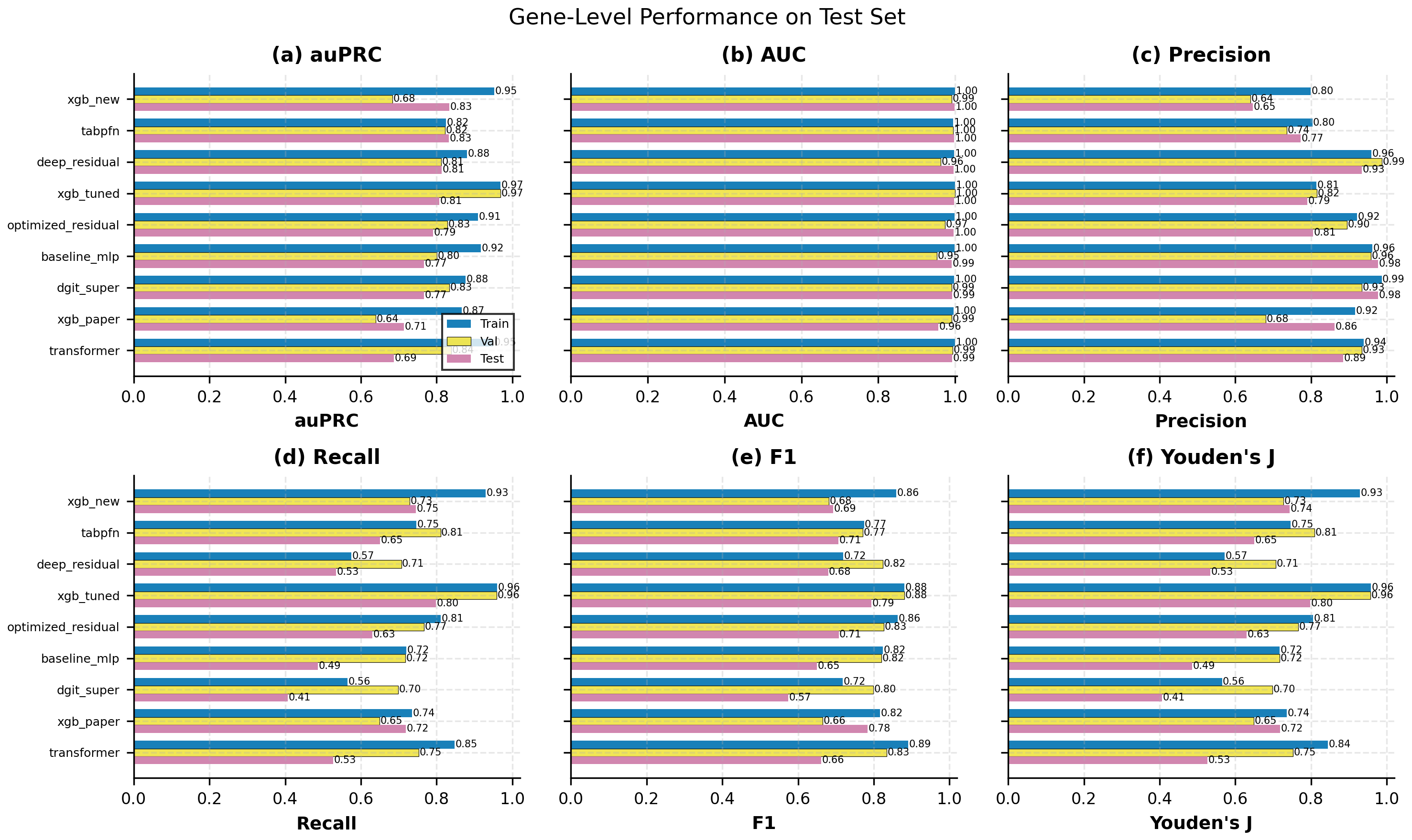
Figure 1: Gene-level performance comparison across training, validation, and test sets. Six metrics are shown: (a) auPRC - primary metric for imbalanced classification, (b) AUC - overall discriminative ability, (c) Precision - positive predictive value, (d) Recall - sensitivity, (e) F1-Score - harmonic mean of precision and recall, (f) Youden's J - optimal threshold selection metric (Sensitivity + Specificity - 1).

Figure 2: Sample-Level Performance on Test Set

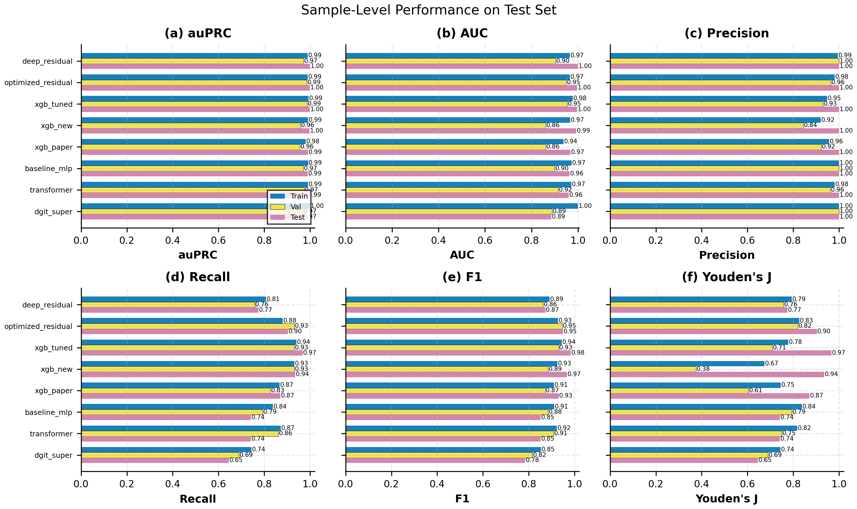
Figure 2: Sample-level performance for circular ecDNA detection. A sample is predicted as circular if any gene is predicted positive. Same six metrics as gene-level are shown.

Figure 3: ROC Space and auROC vs auPRC (Test Set)

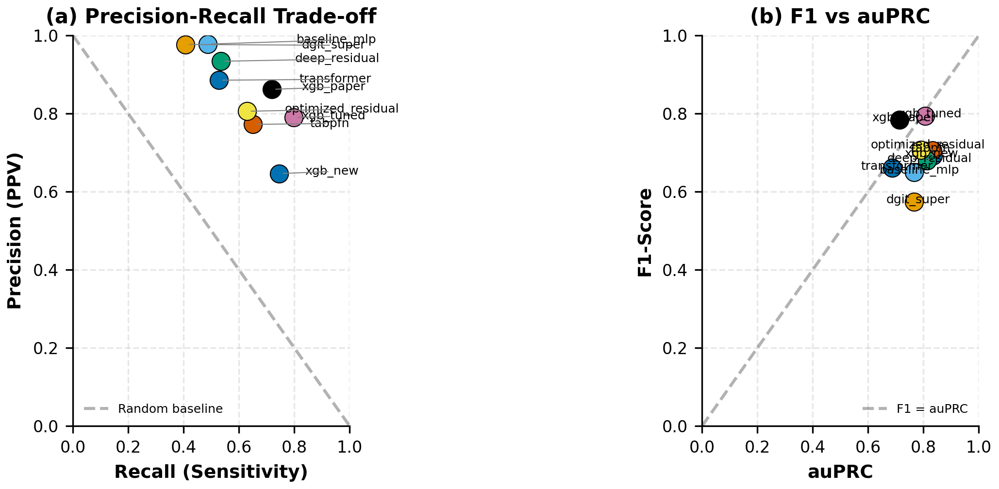
Figure 3: Gene-level trade-off analysis on test set. (a) ROC Space: FPR vs TPR, points closer to top-left indicate better performance. (b) auROC vs auPRC: comparison of two key metrics for imbalanced classification.

Figure 4: Sample-Level ROC Space and auROC vs auPRC (Test Set)

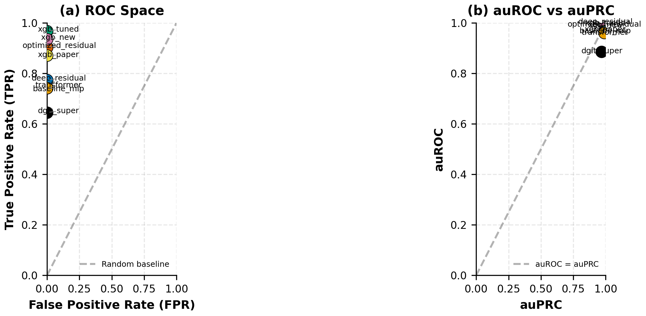
Figure 4: Sample-level trade-off analysis on test set. (a) ROC Space: FPR vs TPR, all models achieve perfect specificity (FPR=0). (b) auROC vs auPRC: comparison of two key metrics.

Figure 5: Multi-dimensional Performance Radar (Test Set)

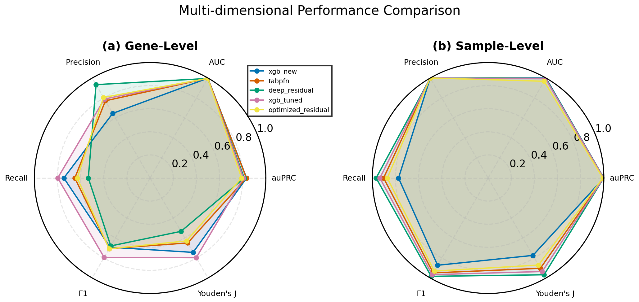
Figure 5: Multi-dimensional performance comparison of top 5 models on test set. (a) Gene-level radar chart. (b) Sample-level radar chart. Larger area indicates better overall performance.

Figure 6: Gene-Level Model Performance Heatmap (Test Set)

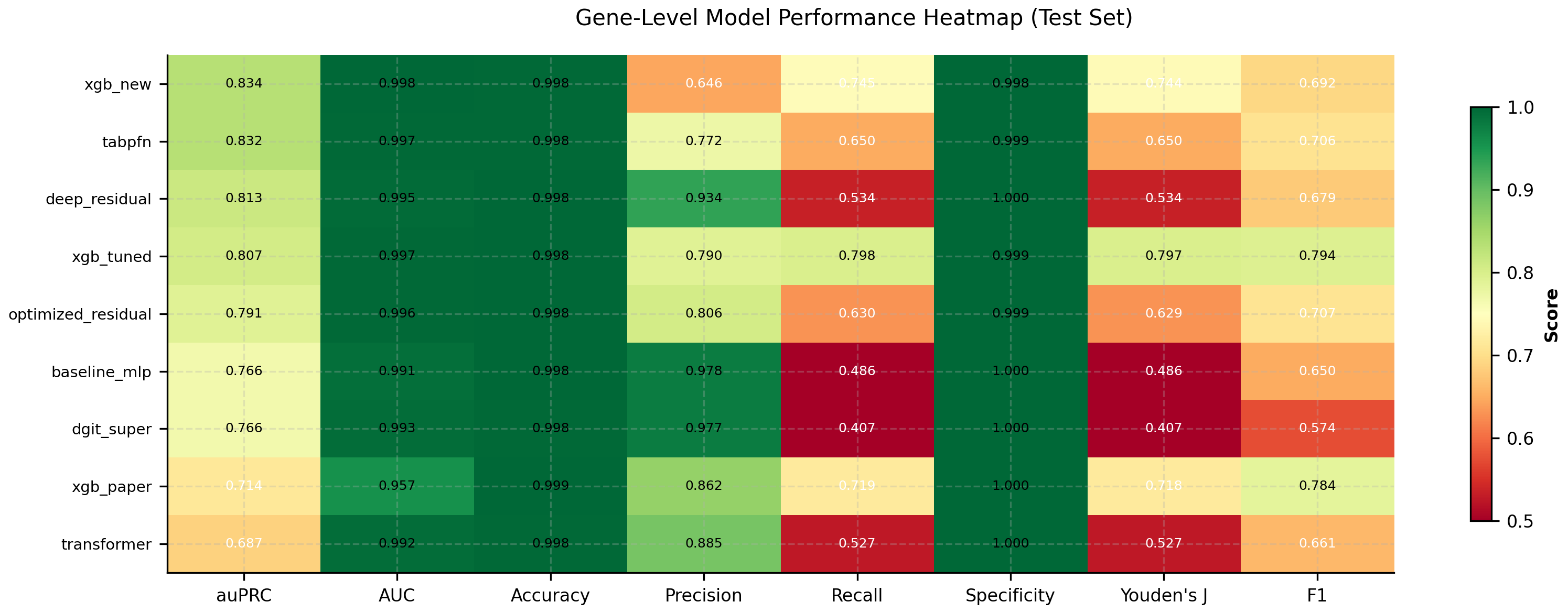
Figure 6: Gene-level model performance heatmap on test set. Eight metrics are compared: auPRC, AUC, Accuracy, Precision, Recall, Specificity, Youden's J, and F1. Darker green indicates better performance.

Figure 7: Sample-Level Model Performance Heatmap (Test Set)

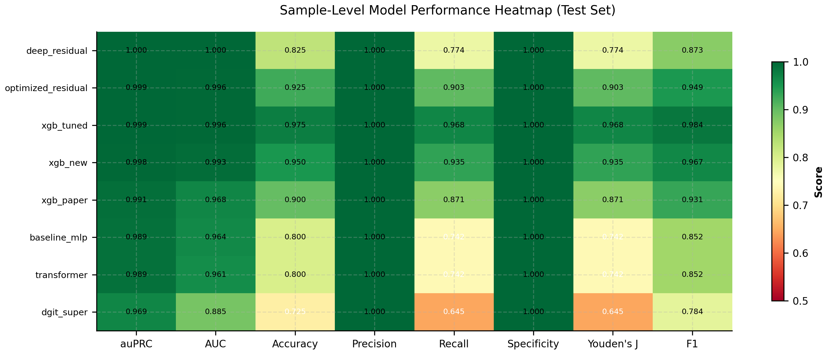
Figure 7: Sample-level model performance heatmap on test set. Eight metrics are compared: auPRC, AUC, Accuracy, Precision, Recall, Specificity, Youden's J, and F1. Darker green indicates better performance.

Test Set Performance (Primary Evaluation)

Model	auPRC	AUC	Precision	Recall	Specificity	F1-Score
xgb_new	0.8339	0.9980	0.6463	0.7454	0.9985	0.6923
tabpfn	0.8323	0.9971	0.7723	0.6504	0.9993	0.7061
deep_residual	0.8132	0.9953	0.9338	0.5339	0.9999	0.6794
xgb_tuned	0.8065	0.9970	0.7900	0.7982	0.9992	0.7941
optimized_residual	0.7906	0.9962	0.8058	0.6300	0.9994	0.7072
baseline_mlp	0.7663	0.9910	0.9777	0.4864	1.0000	0.6497
dgit_super	0.7662	0.9926	0.9768	0.4068	1.0000	0.5744
xgb_paper	0.7138	0.9566	0.8620	0.7186	0.9996	0.7838
transformer	0.6875	0.9922	0.8854	0.5268	0.9997	0.6605

Complete Performance Comparison

Training Set Performance

Model	auPRC	AUC	Precision	Recall	Specificity	F1-Score
baseline_mlp	0.9170	0.9983	0.9624	0.7202	0.9999	0.8239
deep_residual	0.8807	0.9972	0.9599	0.5749	0.9999	0.7191
dgit_super	0.8770	0.9978	0.9867	0.5649	1.0000	0.7185
optimized_residual	0.9098	0.9984	0.9219	0.8112	0.9998	0.8630
tabpfn	0.8246	0.9953	0.8036	0.7467	0.9994	0.7741
transformer	0.9503	0.9993	0.9394	0.8473	0.9998	0.8910
xgb_new	0.9519	0.9993	0.7987	0.9299	0.9992	0.8593
xgb_paper	0.8660	0.9957	0.9171	0.7357	0.9998	0.8164
xgb_tuned	0.9685	0.9998	0.8137	0.9594	0.9992	0.8806

Validation Set Performance

Model	auPRC	AUC	Precision	Recall	Specificity	F1-Score
baseline_mlp	0.8005	0.9530	0.9586	0.7169	0.9999	0.8203
deep_residual	0.8121	0.9621	0.9873	0.7067	1.0000	0.8238
dgit_super	0.8340	0.9906	0.9338	0.6984	0.9998	0.7991
optimized_residual	0.8283	0.9741	0.8955	0.7672	0.9997	0.8264
tabpfn	0.8228	0.9952	0.7360	0.8103	0.9989	0.7714
transformer	0.8393	0.9934	0.9348	0.7532	0.9998	0.8342
xgb_new	0.6838	0.9914	0.6403	0.7286	0.9985	0.6816
xgb_paper	0.6395	0.9905	0.6803	0.6497	0.9989	0.6646
xgb_tuned	0.9684	0.9997	0.8154	0.9580	0.9992	0.8810

Test Set Performance

Model	auPRC	AUC	Precision	Recall	Specificity	F1-Score
baseline_mlp	0.7663	0.9910	0.9777	0.4864	1.0000	0.6497
deep_residual	0.8132	0.9953	0.9338	0.5339	0.9999	0.6794
dgit_super	0.7662	0.9926	0.9768	0.4068	1.0000	0.5744
optimized_residual	0.7906	0.9962	0.8058	0.6300	0.9994	0.7072
tabpfn	0.8323	0.9971	0.7723	0.6504	0.9993	0.7061
transformer	0.6875	0.9922	0.8854	0.5268	0.9997	0.6605
xgb_new	0.8339	0.9980	0.6463	0.7454	0.9985	0.6923
xgb_paper	0.7138	0.9566	0.8620	0.7186	0.9996	0.7838
xgb_tuned	0.8065	0.9970	0.7900	0.7982	0.9992	0.7941

Sample-Level Performance (Circular Detection)

Sample-level evaluation determines whether a sample contains circular ecDNA. A sample is predicted as circular if any gene in the sample is predicted positive.

Test Set Sample-Level Performance

Model	auPRC	AUC	Accuracy	Precision	Recall	Specificity	Youden's J	F1	Samples
deep_residual	1.0000	1.0000	0.8250	1.0000	0.7742	1.0000	0.7742	0.8727	40
optimized_residual	0.9990	0.9964	0.9250	1.0000	0.9032	1.0000	0.9032	0.9492	40
xgb_tuned	0.9990	0.9964	0.9750	1.0000	0.9677	1.0000	0.9677	0.9836	40
xgb_new	0.9979	0.9928	0.9500	1.0000	0.9355	1.0000	0.9355	0.9667	40
xgb_paper	0.9913	0.9677	0.9000	1.0000	0.8710	1.0000	0.8710	0.9310	40
baseline_mlp	0.9894	0.9642	0.8000	1.0000	0.7419	1.0000	0.7419	0.8519	40
transformer	0.9891	0.9606	0.8000	1.0000	0.7419	1.0000	0.7419	0.8519	40
dgit_super	0.9686	0.8853	0.7250	1.0000	0.6452	1.0000	0.6452	0.7843	40

Validation Set Sample-Level Performance

Model	auPRC	AUC	Accuracy	Precision	Recall	Specificity	Youden's J	F1	Samples
baseline_mlp	0.9712	0.9004	0.8421	1.0000	0.7931	1.0000	0.7931	0.8846	38
deep_residual	0.9725	0.9042	0.8158	1.0000	0.7586	1.0000	0.7586	0.8627	38
dgit_super	0.9679	0.8889	0.7632	1.0000	0.6897	1.0000	0.6897	0.8163	38
optimized_residual	0.9856	0.9502	0.9211	0.9643	0.9310	0.8889	0.8199	0.9474	38
transformer	0.9742	0.9157	0.8684	0.9615	0.8621	0.8889	0.7510	0.9091	38
xgb_new	0.9587	0.8621	0.8158	0.8438	0.9310	0.4444	0.3755	0.8852	38
xgb_paper	0.9558	0.8621	0.8158	0.9231	0.8276	0.7778	0.6054	0.8727	38
xgb_tuned	0.9878	0.9540	0.8947	0.9310	0.9310	0.7778	0.7088	0.9310	38

Training Set Sample-Level Performance

Model	auPRC	AUC	Accuracy	Precision	Recall	Specificity	Youden's J	F1	Samples
baseline_mlp	0.9918	0.9732	0.8766	1.0000	0.8376	1.0000	0.8376	0.9116	308
deep_residual	0.9896	0.9652	0.8506	0.9947	0.8077	0.9865	0.7942	0.8915	308
dgit_super	1.0000	1.0000	0.8052	1.0000	0.7436	1.0000	0.7436	0.8529	308
optimized_residual	0.9900	0.9659	0.8961	0.9810	0.8803	0.9459	0.8263	0.9279	308
transformer	0.9914	0.9715	0.8896	0.9808	0.8718	0.9459	0.8177	0.9231	308
xgb_new	0.9906	0.9670	0.8864	0.9198	0.9316	0.7432	0.6749	0.9257	308
xgb_paper	0.9808	0.9384	0.8701	0.9575	0.8675	0.8784	0.7459	0.9103	308
xgb_tuned	0.9935	0.9778	0.9156	0.9483	0.9402	0.8378	0.7780	0.9442	308

Overfitting Analysis

Model	Train-Val auPRC Gap	Severity	Precision Gap	Recall Gap
baseline_mlp	0.1165	⚠️ medium	0.0039	0.0033
deep_residual	0.0686	✅ low	-0.0274	-0.1319
dgit_super	0.0430	✅ low	0.0528	-0.1335
optimized_residual	0.0815	⚠️ medium	0.0265	0.0440
tabpfn	0.0018	✅ low	0.0676	-0.0636
transformer	0.1111	⚠️ medium	0.0046	0.0941
xgb_new	0.2681	❌ high	0.1583	0.2013
xgb_paper	0.2265	❌ high	0.2369	0.0860
xgb_tuned	0.0001	✅ low	-0.0017	0.0014

Best Model Recommendations

Metric	Best Model	Value
Best auPRC	xgb_new	0.8339
Best AUC	xgb_new	0.9980
Best F1-Score	xgb_tuned	0.7941
Best Precision	baseline_mlp	0.9777
Best Recall	xgb_tuned	0.7982
Best Generalization	xgb_tuned	Gap: 0.0001
Best Sample-Level auPRC	deep_residual	1.0000

Usage Guidelines

Metric Selection for Different Scenarios

While auPRC (Area under Precision-Recall Curve) is the primary optimization target for gene-level ecDNA prediction due to class imbalance, users should select metrics based on their specific needs:

Scenario	Recommended Metric	Rationale
High-confidence predictions	Precision	Minimize false positives; use when follow-up validation is expensive
Comprehensive detection	Recall	Maximize true positive detection; use when missing ecDNA is costly
Balanced performance	F1-Score	Harmonic mean of precision and recall; good general-purpose metric
Overall discriminative ability	auPRC	Robust to class imbalance; recommended for gene-level modeling
Sample-level detection	Sample-Level auPRC, Precision, Recall	For determining if a sample contains circular ecDNA; consider precision/recall trade-offs

Practical Recommendations

1. For research validation: Use high-precision models (e.g., baseline_mlp with 97.77% precision) to minimize false positives in downstream experiments.
2. For screening applications: Use high-recall models (e.g., xgb_new with 74.54% recall) to capture most ecDNA-positive genes.
3. For balanced applications: Consider F1-score optimized models (e.g., xgb_paper with 78.38% F1) for a good trade-off.
4. For sample-level detection: All models achieve >98% sample-level auPRC, making them reliable for detecting ecDNA-containing samples.

Architecture Details

baseline_mlp

• Type: BaselineMLP

• Description: Multi-Layer Perceptron

• Structure: 57→128→64→1

• Key Features: Fully connected layers, Non-linear activation

• Suitable For: Baseline model, quick training

• Loss Function: BCEWithLogitsLoss

• Optimizer: Adam (lr=0.001, weight_decay=0.0001)

deep_residual

• Type: DeepResidual

• Description: Residual Network

• Structure: 57→128(ResNet)→1

• Key Features: Residual connections, Skip connections

• Suitable For: Deep feature learning

• Loss Function: BCEWithLogitsLoss

• Optimizer: AdamW (lr=0.001, weight_decay=0.01)

dgit_super

• Type: DGITSuper

• Description: DGITSuper Model

• Structure: 57→192→Transformer(3 layers)→1

• Key Features:

• Suitable For: Custom model

• Loss Function: MultiTaskFocalLoss

• Optimizer: AdamW (lr=0.001, weight_decay=0.01)

optimized_residual

• Type: OptimizedResidual

• Description: Residual Network

• Structure: 57→128(ResNet)→1

• Key Features: Residual connections, Skip connections

• Suitable For: Deep feature learning

• Loss Function: BCEWithLogitsLoss

• Optimizer: AdamW (lr=0.001, weight_decay=0.01)

tabpfn

• Type: Ensemble

• Description: Ensemble Model

• Structure: 57→...→1

• Key Features: Multi-model fusion, Weighted voting

• Suitable For: Robust prediction, reduced overfitting

• Loss Function: Unknown

• Optimizer: Unknown (lr=0.0, weight_decay=0.0)

transformer

• Type: Transformer

• Description: Transformer Attention Model

• Structure: 57→128(embed)→Transformer(3 layers)→1

• Key Features: Self-attention mechanism, LayerNorm, GELU activation

• Suitable For: Feature interaction learning

• Loss Function: BCEWithLogitsLoss

• Optimizer: AdamW (lr=0.001, weight_decay=0.01)

xgb_new

• Type: XGBNew

• Description: XGBoost Gradient Boosting

• Structure: Gradient Boosted Trees (57 features, max_depth=6)

• Key Features: Tree-based ensemble, Feature importance, Native missing value handling

• Suitable For: Tabular data, interpretable predictions

• Loss Function: LogLoss (optimizes auPRC)

• Optimizer: Gradient Boosting (lr=0.05, weight_decay=2.1)

xgb_paper

• Type: XGB11

• Description: XGBoost Gradient Boosting

• Structure: Gradient Boosted Trees (57 features, max_depth=4)

• Key Features: Tree-based ensemble, Feature importance, Native missing value handling

• Suitable For: Tabular data, interpretable predictions

• Loss Function: LogLoss (optimizes auPRC)

• Optimizer: Gradient Boosting (lr=0.1, weight_decay=1)

xgb_tuned

• Type: xgb_tuned

• Description: XGBoost Gradient Boosting

• Structure: Gradient Boosted Trees (68 features, max_depth=7)

• Key Features: Tree-based ensemble, Feature importance, Native missing value handling

• Suitable For: Tabular data, interpretable predictions

• Loss Function: LogLoss (optimizes auPRC)

• Optimizer: Gradient Boosting (lr=0.03672687007849265, weight_decay=6.71081718945088)

Statistical Considerations

Evaluation Metrics

• auPRC (Area under Precision-Recall Curve): Primary metric for imbalanced classification. More informative than AUC when positive class is rare (~0.35% in this dataset).

• AUC (Area under ROC Curve): Measures overall discriminative ability.

• Precision: Proportion of predicted positives that are true positives.

• Recall (Sensitivity): Proportion of actual positives correctly identified.

• F1-Score: Harmonic mean of Precision and Recall.

Sample-Level vs Gene-Level Evaluation

• Gene-Level: Each gene is evaluated independently for ecDNA presence.
• Sample-Level: A sample is predicted as circular if any gene is predicted positive. This reflects the clinical question: 'Does this sample contain circular ecDNA?'

Class Imbalance

At the gene level, the dataset exhibits severe class imbalance (positive rate ~0.35%). However, at the sample level, the positive rate is higher (~76%) as samples were pre-selected based on ecDNA presence. This presents different challenges for model training and evaluation at each level. Models were trained using specialized loss functions and techniques to handle the gene-level imbalance effectively.

Conclusions

Among the 9 models evaluated, xgb_new achieved the highest gene-level test auPRC of 0.8339, demonstrating superior performance for ecDNA prediction on this challenging imbalanced dataset.

Key Findings

1. Best Overall Performance: xgb_new (auPRC: 0.8339, AUC: 0.9980)
2. Best F1-Score: xgb_tuned (F1: 0.7941), balancing precision and recall
3. Best Generalization: xgb_tuned (train-val gap: 0.0001)

Model Architecture Insights

• XGBoost vs Neural Networks: XGBoost models (best: xgb_new, auPRC: 0.8339) outperformed neural network models (best: tabpfn, auPRC: 0.8323) on gene-level prediction, likely due to better handling of tabular data and feature interactions.

• Sample-Level Detection: All models achieved >98% sample-level auPRC, indicating excellent performance for the clinical task of identifying samples containing circular ecDNA.

Clinical Implications

The high sample-level performance (auPRC > 0.98) suggests these models are suitable for clinical screening applications. The gene-level performance varies, allowing users to select models based on their specific precision/recall requirements.

Methods

Data Splitting

Samples were stratified by positive sample count per patient to ensure balanced distribution across training, validation, and test sets. The splitting was performed at the sample level (not gene level) to prevent data leakage.

Model Training

Neural network models were trained using PyTorch, while XGBoost models were trained using the XGBoost library. The following common practices were applied:

• Early stopping based on validation auPRC with patience of 5-50 epochs
• Learning rate scheduling (ReduceLROnPlateau or CosineAnnealingWarmRestarts for neural networks)
• Gradient clipping for neural network training stability
• Model checkpointing to save best performing weights

Limitations

1. Dataset Size: The dataset contains 386 samples, which is relatively small for deep learning models. Larger datasets could improve model generalization.

2. Class Imbalance: Gene-level positive rate (~0.35%) creates challenges for model training, potentially biasing predictions toward the majority class.

3. Sample Selection Bias: Samples were pre-selected based on ecDNA presence, which may not reflect the true prevalence in clinical populations.

4. External Validation: Models were evaluated on a single dataset. External validation on independent datasets is needed to confirm generalizability.

5. Feature Engineering: The current feature set (57-68 features) may not capture all relevant biological signals. Additional genomic features could improve performance.

---

Report generated by OTK Model Analyzer